
Both packages ship a simulated tissue section with a known answer, used by the examples and the tests. It plays the role of a planted signal: each gene of the analyzed cell type has a known density-expression correlation ρ, so a fit can be checked against the truth.
Contents
- 7,449 cells of one tissue section, one row per cell. The section is an irregular, lobed shape inside the window [0, 6] x [0, 4], so the analysis needs a tissue boundary.
- Columns
xandy(coordinates),celltype, andgeneA,geneBandgeneC(counts). - 3,449
Tumorcells, the population analyzed, with true density-expression correlations ρ = 0.6 forgeneA, 0 forgeneBand -0.6 forgeneC. - 4,000
Othercells, which only delineate the tissue; their counts carry no signal.
Load the data
library(DenMark)
toy <- denmark_toy_data()
dim(toy)
#> [1] 7449    6
head(toy)
#>          x        y celltype geneA geneB geneC
#> 1 4.958866 2.517796    Tumor     3     1     1
#> 2 3.398667 1.109772    Tumor     2     1     4
#> 3 2.060565 2.566543    Tumor     1     3     3
#> 4 1.463342 2.365366    Tumor     3     0     4
#> 5 5.085220 2.566559    Tumor    10     1     1
#> 6 2.149059 1.976934    Tumor     0     8     1
table(toy$celltype)
#>
#> Other Tumor
#> 4000 3449How it was made
data-raw/make_toy_data.R simulates the data with
denmark_simulate(rho = c(geneA = 0.6, geneB = 0, geneC = -0.6),
                 width = 6, height = 4, n_cells = 5000, seed = 1,
                 tissue = "irregular", n_other = 4000, celltype = "Tumor")
and writes inst/extdata/denmark_toy.csv.gz, with the
coordinates rounded to six decimals. This is the simulation of
Tutorial_DenMark.Rmd, where the analyzed cell type is
labeled Invasive_Tumor. n_cells is an upper limit: the
thinned point pattern holds 3,449 Tumor cells, and all of them are kept.
The Python package ships a copy of the same file as
python/denmark/data/denmark_toy.csv.gz, and a test checks
that the two are identical. The script also writes the Stan data that R
builds for geneA of the Tumor cells, against which the
tests check Python: python/tests/data/toy_stan_data.json
without a boundary, and
python/tests/data/toy_stan_data_boundary.json with the
alpha-shape boundary of all cells, together with its alpha, the tissue
area and the area and type of every grid cell.
denmark_simulate() follows the DenMark data-generating
process. Candidate locations are drawn uniformly over the window and,
with tissue = "irregular", kept only inside a lobed tissue
outline. The Tumor cells are an inhomogeneous Poisson process obtained
by thinning the candidates, with log intensity a11 w1(s) up to a
constant, where w1 is a smooth zero-mean Gaussian field of approximately
Matérn-3/2 covariance and length-scale 1. The count of gene k in a Tumor
cell at location s is Poisson with log mean
beta1 + sigma2 (ρ_k w1(s) + sqrt(1 - ρ_k^2) w2k(s)),
where w2k is a second, gene-specific field. The defaults are a11 = 1,
sigma2 = 0.8 and beta1 = 0.5. The fields are standardized, and each w2k
is orthogonalized against w1, on a regular lattice over the tissue, so
the spatial correlation of the two fields equals ρ_k. The Other cells
are drawn from the candidates that the thinning rejected, so they are
densest where the Tumor cells are sparse; their counts are Poisson with
mean 0.3. Python’s simulate() follows the same process with
numpy’s generator and does not reproduce the R draws, which is why the
toy data are shared as a file.
Tissue boundary and grid
The tissue boundary is the alpha shape of all cells, Tumor and Other. On the 10 x 10 grid of the examples, each grid cell is interior, boundary or exterior to the tissue, and the exterior grid cells are left out of the model.
tissue <- denmark_alpha_shape(toy$x, toy$y)
c(alpha = attr(tissue, "alpha"), area = as.numeric(sf::st_area(tissue)))
#>     alpha      area
#> 0.1068794 8.5385318
tumor <- subset(toy, celltype == "Tumor", select = -celltype)
g <- buildgridpp(grid_size = 10, dataset = tumor, gene = "geneA", boundary = tissue)
table(g$grid$type)
#>
#> boundary exterior interior
#>       36       18       46
plot_denmark_boundary(toy, tissue, grid = g, highlight = toy$celltype == "Tumor")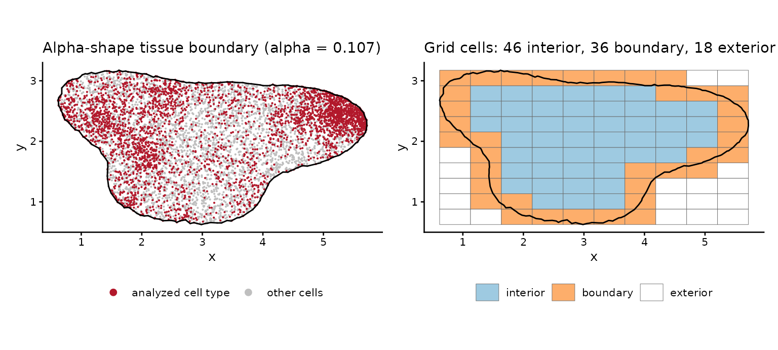
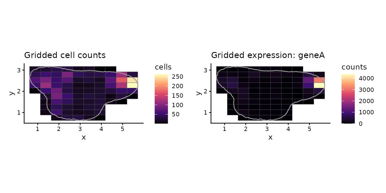
Fits against the truth
The settings below are kept short so the page builds quickly: a 10 x 10 grid, 10 x 10 basis functions and two chains of 500 warm-up and 500 sampling iterations. An analysis uses the default sampler settings: four chains of 1,000 warm-up and 1,000 sampling iterations.
The scan
scan <- denmark_scan(tumor, boundary = tissue, grid_size = 10, basis = 10,
                     chains = 2, iter_warmup = 500, iter_sampling = 500, seed = 2024)
scan$true_rho <- c(geneA = 0.6, geneB = 0, geneC = -0.6)[scan$gene]
scan[, c("gene", "true_rho", "rho_mean", "rho_lower", "rho_upper", "class", "converged")]
#>    gene true_rho   rho_mean  rho_lower  rho_upper   class converged
#> 1 geneA      0.6  0.6379898  0.3456775  0.8585084     PCG      TRUE
#> 2 geneB      0.0  0.1449796 -0.2231820  0.4902050 not DCG     FALSE
#> 3 geneC     -0.6 -0.6001581 -0.8268561 -0.3320357     NCG     FALSE
plot_denmark_scan(scan)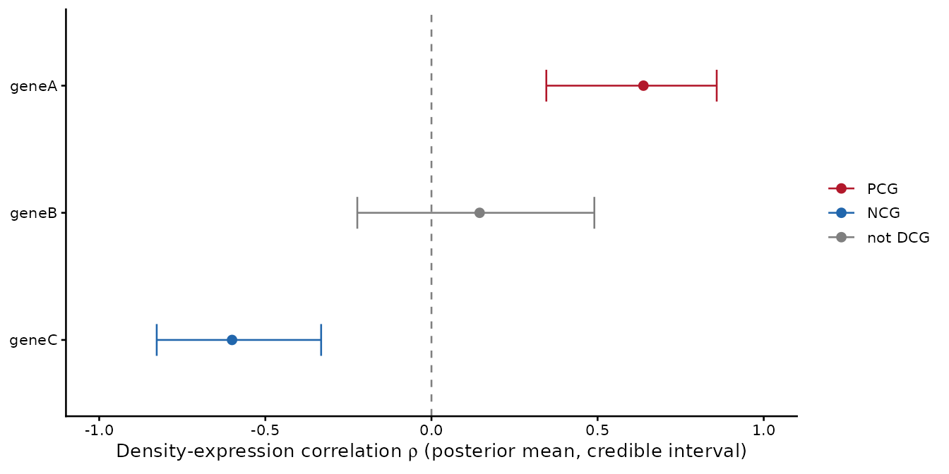
import denmark as dm

toy = dm.datasets.load_toy()
tissue = dm.alpha_shape(toy["x"], toy["y"])
tumor = toy[toy["celltype"] == "Tumor"].drop(columns="celltype")
scan = dm.scan_genes(tumor, boundary=tissue, grid_size=10, basis=10, chains=2,
                     iter_warmup=500, iter_sampling=500, seed=2024)
print(scan[["gene", "rho_mean", "rho_lower", "rho_upper", "class", "converged"]])