Get started in R

DenMark measures how gene expression depends on local cell density in single-cell resolution spatial transcriptomics data. Cell locations form a point pattern and the counts of a gene are its marks. After the cells are binned on a regular grid over the tissue, the DenMark model for grid cell $g$ with area $|g|$ inside the tissue, cell count $Y(g)$ and summed expression $M(g)$ is

$$\begin{aligned} Y(g) &\sim \text{Poisson}\{\lambda_1(g)\}, & \log\lambda_1(g) &= \log|g| + \beta_0 + a_{11}w_1(g),\\ M(g)\mid Y(g) &\sim \text{Poisson}\{\lambda_2(g)\}, & \log\lambda_2(g) &= \beta_1 + \log\{Y(g)+0.05\} + a_{21}w_1(g) + a_{22}w_2(g), \end{aligned}$$

where $w_1$ and $w_2$ are independent unit-variance Gaussian processes with Matern-3/2 covariance, approximated by Hilbert space basis functions (HSGP). With $a_{11} = \sigma_1$, $a_{21} = \sigma_2\rho$ and $a_{22} = \sigma_2\sqrt{1-\rho^2}$, the parameter $\rho$ (Astar[2,1] in Stan) is the density-expression correlation.

This vignette runs the workflow on the bundled toy data, where the true correlations are known, so every estimate can be checked against the truth.

Installation

DenMark is installed from the StaGILL R-universe. It fits its models with Stan through cmdstanr, which needs a working CmdStan installation, and computes the tissue boundary with sf. Install them once:

install.packages(c("DenMark", "sf", "patchwork"),
                 repos = c("https://stagill.r-universe.dev",
                           "https://stan-dev.r-universe.dev", getOption("repos")))
cmdstanr::install_cmdstan()

The toy data

denmark_toy_data() returns a tissue section simulated by denmark_simulate(): 7,449 cells in an irregular, lobed section inside a 6 x 4 window, one row per cell, with the cell type and the counts of three genes. The 3,449 Tumor cells are the population analyzed; their true density-expression correlations are 0.6 for geneA, 0 for geneB and -0.6 for geneC. The 4,000 Other cells only delineate the tissue.

library(DenMark)
library(ggplot2)

toy <- denmark_toy_data()
head(toy)
#>          x        y celltype geneA geneB geneC
#> 1 4.958866 2.517796    Tumor     3     1     1
#> 2 3.398667 1.109772    Tumor     2     1     4
#> 3 2.060565 2.566543    Tumor     1     3     3
#> 4 1.463342 2.365366    Tumor     3     0     4
#> 5 5.085220 2.566559    Tumor    10     1     1
#> 6 2.149059 1.976934    Tumor     0     8     1
table(toy$celltype)
#> 
#> Other Tumor 
#>  4000  3449
tumor <- subset(toy, celltype == "Tumor", select = -celltype)
truth <- c(geneA = 0.6, geneB = 0, geneC = -0.6)

ggplot(tumor, aes(x, y, color = geneA)) +
  geom_point(size = 0.6) +
  scale_color_viridis_c(option = "magma") +
  coord_equal() +
  theme_classic()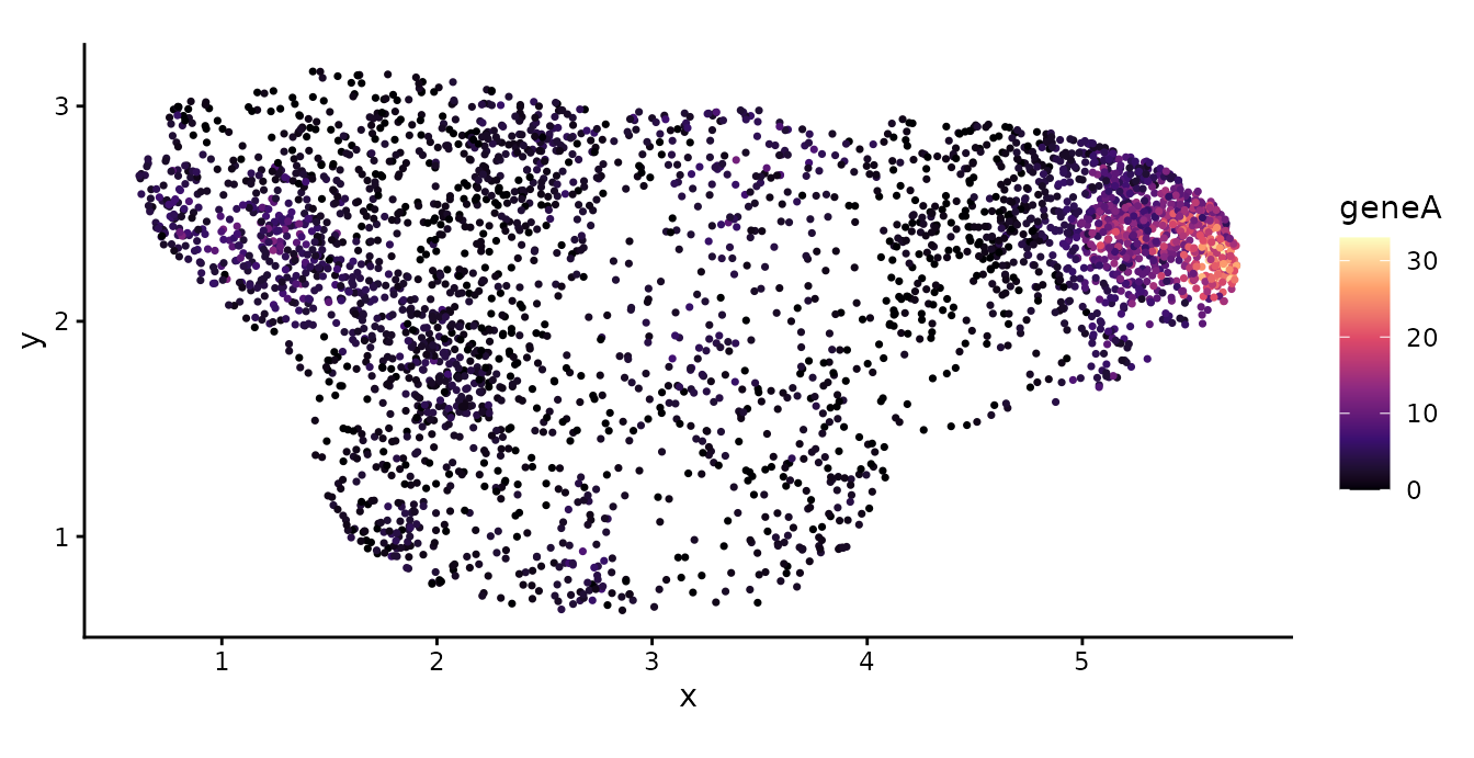

Tissue boundary

A tissue section is rarely a rectangle. If the grid covered the bounding box of the cells, grid cells outside the tissue would hold no cells because there is no tissue there, and the model would read them as regions of low cell density. denmark_alpha_shape() delineates the tissue as an alpha shape: it triangulates the cell locations and keeps every Delaunay triangle whose circumradius is below $\alpha$, by default three times the median Delaunay edge length. The boundary is computed from all cells of the section, not only the Tumor cells, because the region where a Tumor cell could have been observed is the whole tissue.

tissue <- denmark_alpha_shape(toy$x, toy$y)
c(alpha = attr(tissue, "alpha"), area = as.numeric(sf::st_area(tissue)))
#>     alpha      area 
#> 0.1068794 8.5385318

Gridding

buildgridpp() assigns every cell to one grid cell and returns the cell counts $Y(g)$ and the summed expression $M(g)$. Grid cells are ordered with x varying fastest. With boundary, the grid spans the extent of the tissue, and each grid cell is classified as interior (entirely inside the tissue), boundary (partly inside) or exterior, with its area inside the tissue in the column area.

gridded <- buildgridpp(grid_size = 10, dataset = tumor, gene = "geneA",
                       boundary = tissue)
head(gridded$grid)
#>   grid_index i j         x         y  Y  M       area     type
#> 1          1 1 1 0.8713599 0.7530424  0  0 0.00000000 exterior
#> 2          2 2 1 1.3814337 0.7530424  0  0 0.00000000 exterior
#> 3          3 3 1 1.8915075 0.7530424 12 18 0.02704043 boundary
#> 4          4 4 1 2.4015813 0.7530424 29 63 0.09246043 boundary
#> 5          5 5 1 2.9116551 0.7530424 31 78 0.11468348 boundary
#> 6          6 6 1 3.4217289 0.7530424 14 13 0.09659054 boundary
table(gridded$grid$type)
#> 
#> boundary exterior interior 
#>       36       18       46
plot_denmark_boundary(toy, tissue, grid = gridded,
                      highlight = toy$celltype == "Tumor")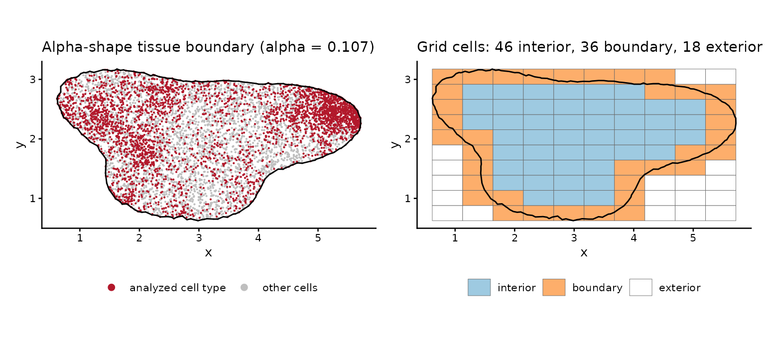

Exterior grid cells are dropped from the model, and boundary grid cells enter with their area inside the tissue, so the area offset $\log|g|$ differs between grid cells. plot_denmark_grid() shows the gridded counts inside the tissue.

plot_denmark_grid(gridded)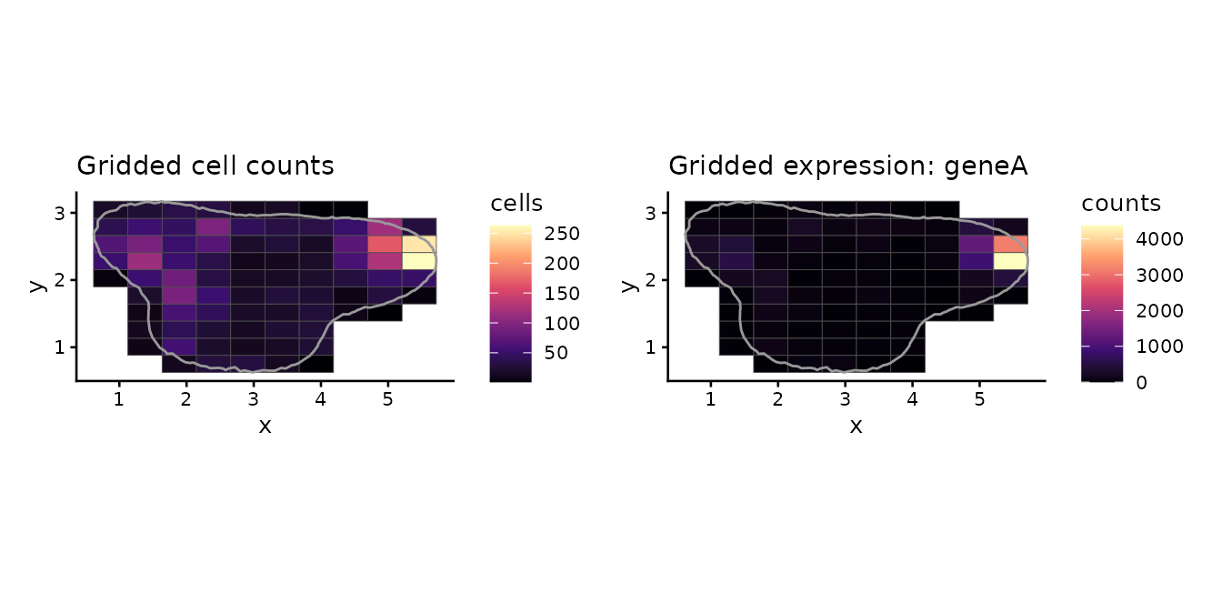

denmark_prepare() builds the Stan input that DenMark() uses: it drops the exterior grid cells, centers the region of interest at the origin, uses the grid centroids as HSGP coordinates and sets the HSGP domain to boundfactor times the half-ranges. With a boundary, log_grid_area holds one value per grid cell in the model.

prep <- denmark_prepare(tumor, gene = "geneA", grid_size = 10, basis = 10,
                        boundfactor = 1.5, boundary = tissue)
str(prep$stan_data[c("n", "mstar", "L", "log_grid_area", "mrange")])
#> List of 5
#>  $ n            : int 82
#>  $ mstar        : int 100
#>  $ L            : num [1:2] 3.83 1.91
#>  $ log_grid_area: num [1:82] -3.61 -2.38 -2.17 -2.34 -4.68 ...
#>  $ mrange       : num 0.933

Fitting the model

DenMark() grids the data, compiles the Stan model once per session and samples. With boundary, it fits the variable-area model DenMark-vararea.stan, the same model with one area offset per grid cell; without it, the bounding box of the cells is gridded with a common grid area. The settings below keep the vignette fast; for real data, use the defaults (four chains of 1,000 warm-up and 1,000 sampling iterations and basis = 25) and check the diagnostics.

fit <- DenMark(tumor, gene = "geneA", boundary = tissue, grid_size = 10,
               basis = 10, boundfactor = 1.5, chains = 2, iter_warmup = 500,
               iter_sampling = 500, seed = 2024, quiet = TRUE)
fit
#> DenMark fit  |  gene geneA
#>   grid 10 x 10 (82 grids, 3449 cells)  |  basis 10  |  boundfactor 1.50
#>   rho (density-expression correlation): 0.638  [95% CrI 0.346, 0.859]
#>   max R-hat 1.009 | min ESS bulk 331 | divergences 0 | time 0.82 min
#> 
#>    variable    mean    sd   q2.5    q50 q97.5 rhat ess_bulk
#>       beta0  5.5811 0.353  4.861 5.6016 6.202 1.01      700
#>       beta1 -0.0311 0.542 -1.293 0.0393 0.828 1.01      648
#>      ell[1]  0.6162 0.154  0.385 0.5991 0.987 1.01      428
#>      ell[2]  0.7830 0.268  0.414 0.7383 1.433 1.01      561
#>  Astar[2,1]  0.6380 0.133  0.346 0.6522 0.859 1.00      520
#>    sigma[1]  1.0171 0.216  0.705 0.9753 1.552 1.00      457
#>    sigma[2]  1.3610 0.319  0.869 1.3105 2.099 1.01      331

Posterior summaries

denmark_summary() reports the intercepts, the length-scales ell[1] and ell[2], $\rho$ and the field standard deviations, with R-hat and effective sample sizes.

denmark_summary(fit)[, c("variable", "mean", "sd", "q2.5", "q97.5",
                         "rhat", "ess_bulk")]
#>     variable        mean        sd       q2.5     q97.5     rhat ess_bulk
#> 1      beta0  5.58114090 0.3526443  4.8607692 6.2016856 1.006094 699.5902
#> 2      beta1 -0.03109354 0.5424765 -1.2934254 0.8279460 1.006202 647.6565
#> 3     ell[1]  0.61620164 0.1535301  0.3848757 0.9867065 1.006640 427.7415
#> 4     ell[2]  0.78302753 0.2675554  0.4142325 1.4326819 1.009326 560.5678
#> 5 Astar[2,1]  0.63798981 0.1331256  0.3456775 0.8585084 1.002078 520.4197
#> 6   sigma[1]  1.01707506 0.2158568  0.7049778 1.5522819 1.002127 457.4781
#> 7   sigma[2]  1.36097278 0.3190100  0.8692649 2.0991409 1.006148 330.6966

denmark_draws() returns one row per posterior draw, including $\rho$. The red line marks the true value.

draws <- denmark_draws(fit)
ggplot(draws, aes(rho)) +
  geom_density(fill = "grey80") +
  geom_vline(xintercept = 0, linetype = 2) +
  geom_vline(xintercept = truth[["geneA"]], color = "#B2182B") +
  xlim(-1, 1) +
  labs(x = expression(rho), y = "Posterior density") +
  theme_classic()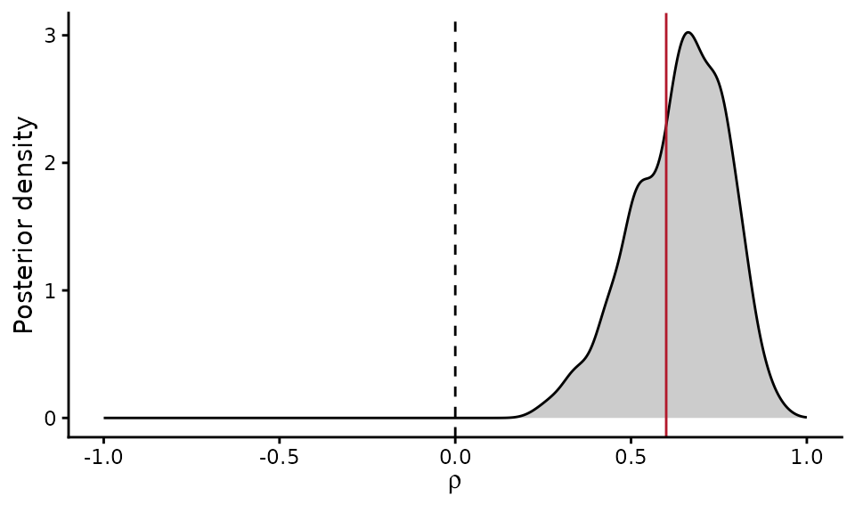

Latent fields

denmark_fields() decomposes, for every grid cell in the model, the log cell intensity $\beta_0 + a_{11}w_1$ and the log expression per cell $\beta_1 + a_{21}w_1 + a_{22}w_2$ into the density field $a_{11}w_1$, the density-shared part of expression $a_{21}w_1$ and the expression-specific part $a_{22}w_2$.

fields <- denmark_fields(fit)
head(fields[, c("grid_index", "Y", "M", "eta1", "a11w1", "eta2", "a21w1", "a22w2")])
#>   grid_index  Y  M     eta1      a11w1       eta2      a21w1     a22w2
#> 1          3 12 18 6.074419  0.4932781 0.51964249  0.4196085 0.1311275
#> 2          4 29 63 5.726415  0.1452738 0.82066851  0.1265022 0.7252598
#> 3          5 31 78 5.423532 -0.1576085 0.91454377 -0.1307803 1.0764177
#> 4          6 14 13 5.033918 -0.5472232 0.03532403 -0.4563928 0.5228104
#> 5          7  1  1 5.439027 -0.1421143 0.02323582 -0.1146863 0.1690156
#> 6         12  8 15 6.291088  0.7099472 0.74137691  0.6021673 0.1703032
plot_denmark_fields(fit, fields = fields)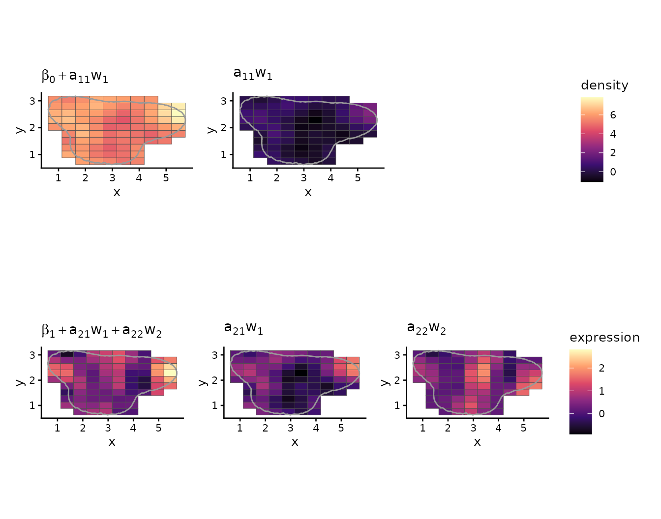

Spatial correlation ranges

denmark_decay() gives the posterior spatial correlation of the density and expression fields as a function of distance, and the practical range, the distance at which the correlation falls to 0.05.

decay <- denmark_decay(fit)
decay$ranges
#>        field     mean   median    lower    upper
#> 1    density 1.687697 1.640848 1.054125 2.702462
#> 2 expression 2.103655 1.961955 1.274218 3.745892
plot_denmark_decay(fit, decay = decay)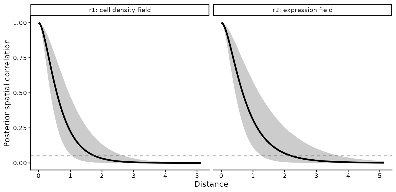

Scanning genes for density-correlated genes

denmark_scan() fits DenMark to each gene and calls it a positively (PCG) or negatively (NCG) density-correlated gene when the 95% credible interval of $\rho$ lies above or below 0, and not a DCG otherwise.

scan <- denmark_scan(tumor, genes = c("geneA", "geneB", "geneC"),
                     boundary = tissue, grid_size = 10, basis = 10,
                     boundfactor = 1.5, chains = 2, iter_warmup = 500,
                     iter_sampling = 500, seed = 2024, verbose = FALSE)
scan[, c("gene", "rho_mean", "rho_lower", "rho_upper", "class", "max_rhat")]
#>    gene   rho_mean  rho_lower  rho_upper   class max_rhat
#> 1 geneA  0.6379898  0.3456775  0.8585084     PCG 1.009326
#> 2 geneB  0.1449796 -0.2231820  0.4902050 not DCG 1.003555
#> 3 geneC -0.6001581 -0.8268561 -0.3320357     NCG 1.020449

plot_denmark_scan(scan)
#> `height` was translated to `width`.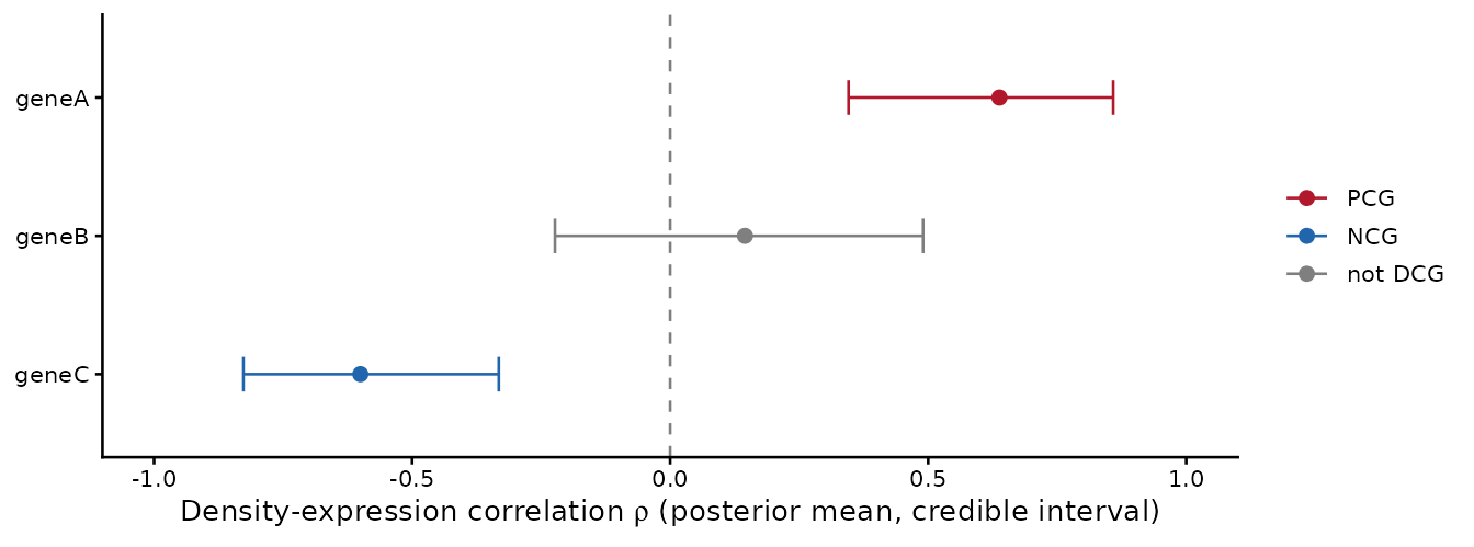

For a full panel, workers = 4 fits four genes at a time, each in its own R session, with the same results as the sequential scan; every fit also runs its chains in parallel, so plan for workers times chains cores. On a cluster, the template in system.file("slurm", package = "DenMark") fits one gene per SLURM array task and then collects the results with denmark_scan().

Checking the estimates against the truth

With true values of 0.6, 0 and -0.6, the expected calls are PCG for geneA, not DCG for geneB and NCG for geneC. The table compares each posterior mean and 95% credible interval with the true $\rho$; covered shows whether the interval contains it. Reading density-correlated genes explains what a call can and cannot tell you, and how to tell a change within the focal cells from a signal of their neighborhood.

check <- data.frame(gene = scan$gene, truth = truth[scan$gene],
                    estimate = scan$rho_mean, lower = scan$rho_lower,
                    upper = scan$rho_upper, class = scan$class,
                    row.names = NULL)
check$covered <- check$lower <= check$truth & check$truth <= check$upper
check
#>    gene truth   estimate      lower      upper   class covered
#> 1 geneA   0.6  0.6379898  0.3456775  0.8585084     PCG    TRUE
#> 2 geneB   0.0  0.1449796 -0.2231820  0.4902050 not DCG    TRUE
#> 3 geneC  -0.6 -0.6001581 -0.8268561 -0.3320357     NCG    TRUE

Using your own data

DenMark needs one row per cell with the coordinates in columns x and y and raw counts in one column per gene. Compute the tissue boundary from all cells of the section, then analyze the cells of one population: filter uninformative genes, fit one gene, then scan the panel; with save_dir, each gene is saved as it finishes and an interrupted scan resumes where it stopped.

cells <- read.csv("cells.csv")   # all cells: x, y, celltype and gene counts
# or from a Seurat object (Xenium, MERSCOPE or CosMx) with cell types in its metadata:
# cells <- denmark_from_seurat(obj, celltype = "celltype")
tissue <- denmark_alpha_shape(cells$x, cells$y)
focal <- subset(cells, celltype == "Tumor", select = -celltype)
genes <- denmark_filter_genes(focal[, setdiff(names(focal), c("x", "y"))])
fit <- DenMark(focal[, c("x", "y", genes[1])], gene = genes[1],
               boundary = tissue, grid_size = 15, basis = 25, boundfactor = 1.5)
dcg <- denmark_scan(focal[, c("x", "y", genes)], boundary = tissue,
                    grid_size = 15, basis = 25, save_dir = "denmark_scan")

denmark_annotate(obj, dcg) writes the estimates, their intervals and the calls back into the Seurat object’s gene metadata. denmark_check_hsgp() compares the posterior length-scales with a rule of thumb for the number of basis functions and the boundary factor, and denmark_save() keeps a fit for later sessions.